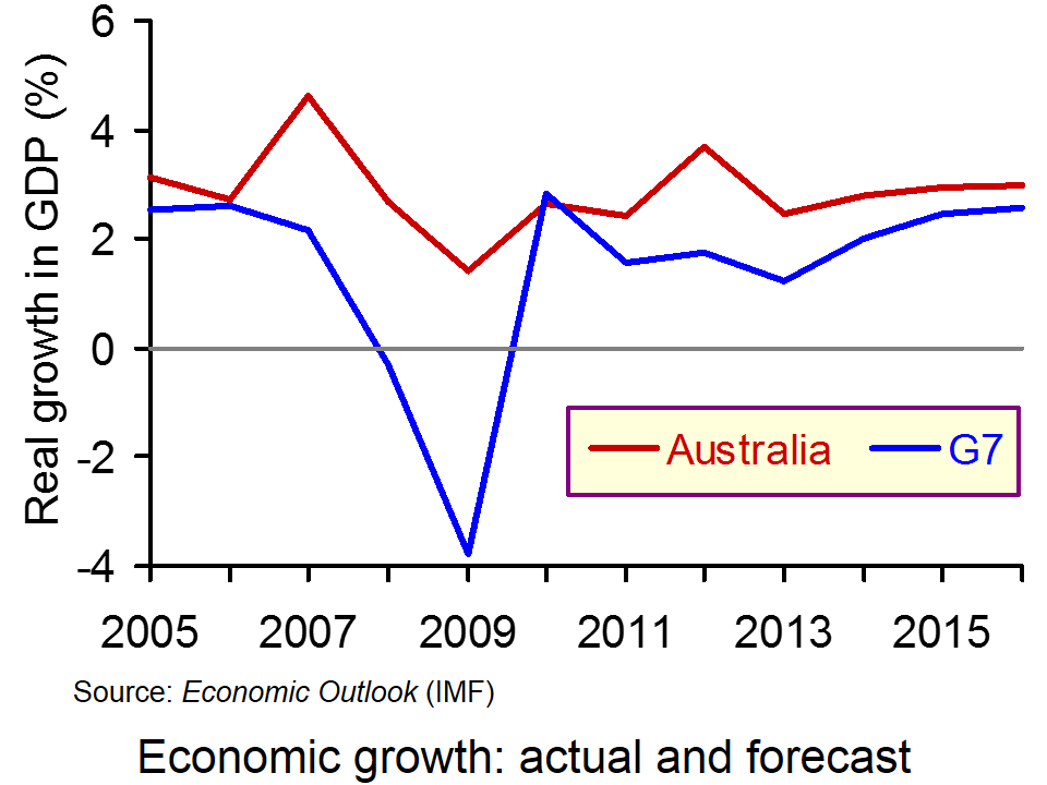
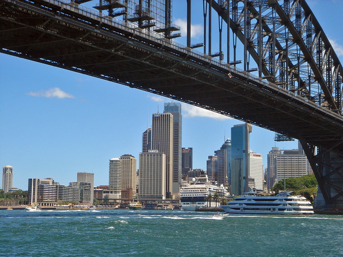
When the rest of the developed world went into recession after the financial crisis of 2007/8, the Australian economy kept growing, albeit at a slightly lower rate (see chart 1: click here for a PowerPoint). Then as the world economy began to grow again after 2009, Australian grow accelerated. Partly this was the result of a strong growth in demand for Australian mineral exports, such as coal, iron ore and bauxite, especially from China and other east Asian countries.
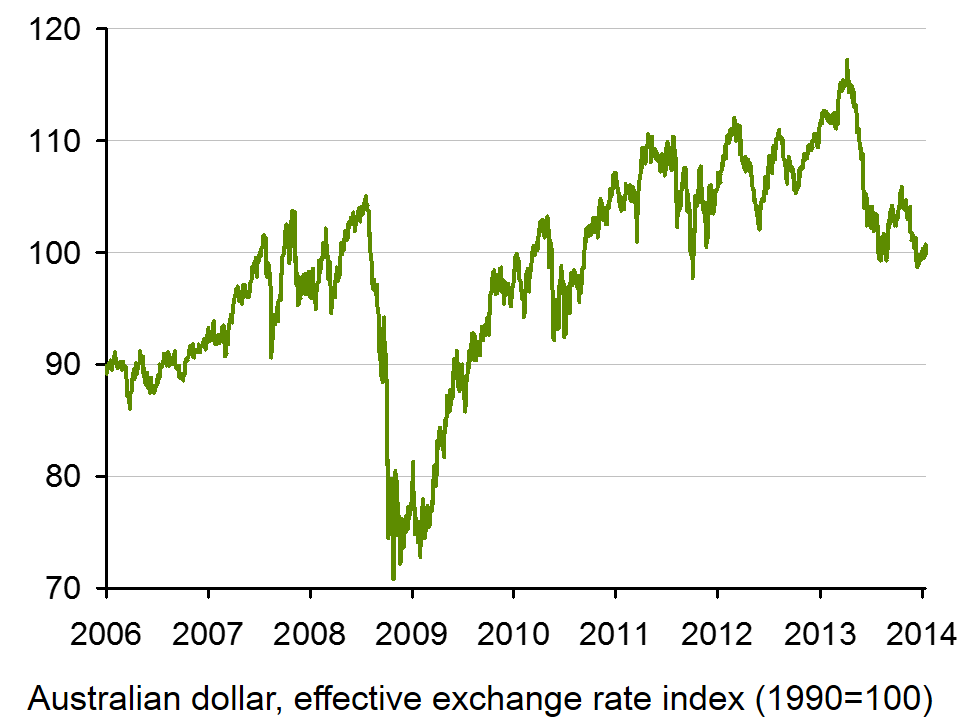
But in 2013, Australian growth slowed and jobs grew by their lowest rate for 17 years. Employment actually fell by 22,600 in December and unemployment was only prevented from rising by a fall in the participation rate. The Australian dollar, which has been depreciating in recent months, fell further on the news about jobs, reaching its lowest level for over two years (see chart 2: click here for a PowerPoint).
Chart 1 Chart 2
The following articles look at the reasons behind Australia’s slowing growth and at possible reactions of the Australian government and the Reserve Bank of Australia (Australia’s central bank). They also look at the link between economic performance and policy on the one hand and the exchange rate on the other.
Why has the Australian dollar been depreciating in recent months?
Why did the Australian dollar fall further on the news that economic growth had slowed and employment had fallen?
Find out what has been happening to commodity prices in the past three years (see Economic Data freely available online and especially site 26) How has this affected (a) the current account of Australia’s balance of payments; (b) the exchange rate of the Australian dollar?
If commodity prices are in US dollars, how is a depreciation of the Australian dollar likely to affect Australia’s balance of payments?
How are possible fiscal and monetary responses in Australia likely to affect the exchange rate of the Australian dollar?
What determines the magnitude of the rise or fall in demand for Australian exports as the world economy grows or declines? How are the determinants of the price and income elasticities of demand for Australian exports relevant to your answer?
It is one year since the election of Shinzo Abe in Japan. He immediately embarked on a radical economic policy to stimulate the Japanese economy, which had suffered from years of stagnation. There have been three parts (or three arrows) to his policy: fiscal policy and monetary policy to stimulate aggregate demand and supply-side policy to increase productivity.
As the previous post explains:
“The first arrow is monetary policy. The Bank of Japan has engaged in extensive quantitative easing through bond purchases in order to drive down the exchange rate (see A J-curve for Japan?), stimulate expenditure and increase the rate of inflation. A target inflation rate of 2% has been set by the Bank of Japan. Part of the problem for the Japanese economy over the years has been stagnant or falling prices. Japanese consumers have got used to waiting to spend in the hope of being able to buy at lower prices. Similarly, Japanese businesses have often delayed stock purchase. By committing to bond purchases of whatever amount is necessary to achieve the 2% inflation target, the central bank hopes to break this cycle and encourage people to buy now rather than later.
The second arrow is fiscal policy. Despite having the highest debt to GDP ratio in the developed world, Japan is embarking on a large-scale programme of infrastructure investment and other public works. The package is worth over $100bn. The expansionary fiscal policy is accompanied by a longer-term plan for fiscal consolidation as economic growth picks up. In the short term, Japan should have no difficulty in financing the higher deficit, given that most of the borrowing is internal and denominated in yen.
The third arrow is supply-side policy. On 5 June, Shinzo Abe unveiled a series of goals his government would like to achieve in order to boost capacity and productivity. These include increasing private-sector investment (both domestic and inward), infrastructure expenditure (both private and public), increasing farmland, encouraging more women to work by improving day-care facilities for children, and deregulation of both goods, capital and labour markets. The prime minister, however, did not give details of the measures that would be introduced to achieve these objectives. More details will be announced in mid-June.”
In the webcast and article below, Linda Yueh, the BBC’s Chief Business Correspondent, considers how effective the policies are proving and the challenges that remain.
Demonstrate on (a) an aggregate demand and supply diagram and (b) a Keynesian 45° line diagram the effects of the three arrows (assuming they are successful) in meeting their objectives.
Why has Japan found it so hard to achieve economic growth over the past 20 years?
How has the Japanese economy performed over the past 12 months?
What lessons can be learnt by the UK and eurozone countries from Japan’s three arrows?
Why is the second arrow problematic, given the size of Japan’s general government debt? Does the proportion of Japanese debt owed overseas affect the argument?
In what ways do the three arrows (a) support each other; (b) conflict with each other?
Why is the structure of the labour market in Japan acting as a break on economic growth? What policies are being, or could be, pursued to tackle these structural problems?
Compared with pre-financial crisis levels, the British pound is significantly weaker when measured against a basket of foreign currencies. In this blog we provide a further update of Appreciating a depreciating pound which was published back in early December 2012. The significance of the depreciation should be seen in the context of the UK as an open, island-economy where the ratio of exports to GDP in 2012 was close to 32%.
The competitiveness of our exports is, in part, affected by the exchange rate. Floating exchange rates are notoriously volatile. For example, some of the articles below show how sensitive the British pound can be latest news on the economy. However, since the autumn of 2007 we have observed a significant depreciation of the UK exchange rate. A depreciation helps to make our exports more competitive abroad and can potentially boost aggregate demand.
Rather than simply focus on bilateral exchange rates and so at the British pound separately against other foreign currencies, we can estimate an average exchange rate against a whole bundle of currencies. The average rate is calculated by weighting the individual exchange rates by the amount of trade between Britain and the other countries. This trade-weighted exchange rate is known as the effective exchange rate.
In analysing the competitiveness of the exchange rate, we can go one step further and adjust for the average (domestic currency) price of our exports relative to the average (foreign currency) price of those goods we import. Therefore, as well as the nominal (actual) effective exchange rate we can calculate a real effective exchange rate. If the average price of our exports rises relative to the average price of imports, the real effective exchange rate rises relative to the nominal rate. It means that we are able to obtain a larger volume of imports from selling a given volume of exports.
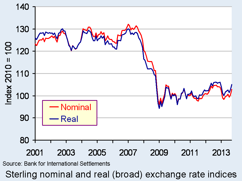
The chart shows the nominal (actual) and real effective exchange rate for the British pound since 2001. The chart shows clearly how from the autumn of 2007 the effective exchange rate fell sharply both in nominal and real terms.
Over the period from July 2007 to January 2009 the nominal effective exchange rate fell by 26.8 per cent while the real effective exchange rate fell by 26.6 per cent. In other words, the British pound depreciated more than one-quarter over an 18-month period. In comparison, the American dollar rose by 5.3 per cent in nominal terms and by 1.9 per cent in real terms. (Click here to download a PowerPoint of the chart.)
If we move the clock forward, we observe an appreciation of the British pound between July 2011 and September 2012. Over this period, the British pound appreciated by 7.0 per cent in nominal terms and by 7.3 per cent in real terms. However, this appreciation had effectively been wiped-out when by March 2013 the nominal rate had depreciated by 6.1 per cent and by 5.6 per cent in real terms. Subsequently, there has been a slight appreciation once more. As of September, the nominal rate had risen by 4.5 per cent and the real rate by 4.8 per cent.
While, as recent figures help to demonstrate, the British pound continues on its roller-coaster ride, there has been a very marked depreciation since the giddy-days prior to the financial crisis. The facts show that when comparing the effective exchange rate in September 2013 with July 2007 the British pound was 21.8 per cent lower in nominal terms and 18.3 per cent in real terms. Over the same period, the US dollar, for example, was only 1.3 per cent lower in nominal terms and 6.1 per cent in real terms. This constitutes a major competitive boost for our exporters. Nonetheless, there remain uncertainty about just how much British exporters can take advantage of this, the amount that it will boost British growth and the impact it will make on the country’s chronic balance of trade deficit in goods which was close to 7 per cent of GDP in 2012.
Explain how the foreign demand for goods and assets generates a demand for British pounds. How will this demand be affected by the foreign currency price of the British pound, i.e. the number of foreign currency units per £1?
Explain how the demand by British residents for foreign goods and assets generates a supply of British pounds. How will this supply be affected by the foreign currency price of the British pound, i.e. the number of foreign currency units per £1?
What factors are likely to shift the demand and supply curves for British pounds on the foreign exchange markets?
Illustrate the effect of a decrease in the demand for British goods and assets on the exchange rate (i.e. the foreign currency price of the British pound) using a demand-supply diagram.
What is the difference between a nominal and a real effective exchange rate? Which of these is a better indicator of the competitiveness of our country’s exports?
What factors are likely to have caused the depreciation of the British pound since 2007?
What is meant by a deficit on the balance of trade in goods?
What relationship exists between the demand and supply of currencies on the foreign exchange markets and the balance of payments?
There has been an interesting debate recently about whether the austerity policies being pursued in the UK are the correct ones. What would have happened if the government had pursued a more expansionary policy? Would the increase in borrowing, at least in the short term, have triggered a financial crisis?
Without austerity policies, would the eurozone crisis have led to a collapse in investor confidence in the UK, especially if Greece had been forced out of the euro?
On the one side, Kenneth Rogoff argues that increasing the UK’s budget deficit would have been dangerous and could have led to a flight from the pound. Generally, but with some reservations, he supports the fiscal policies that have been pursued by the Coalition.
I am certainly not arguing that the UK or other advanced countries handled the post-crisis period perfectly. There should have been more infrastructure spending, even more aggressive monetary policy and probably more ruthless bank restructuring. But there has to be a balance between stimulus and stability. To assume we always knew things would calm down, and to retrospectively calibrate policy advice accordingly, is absurd
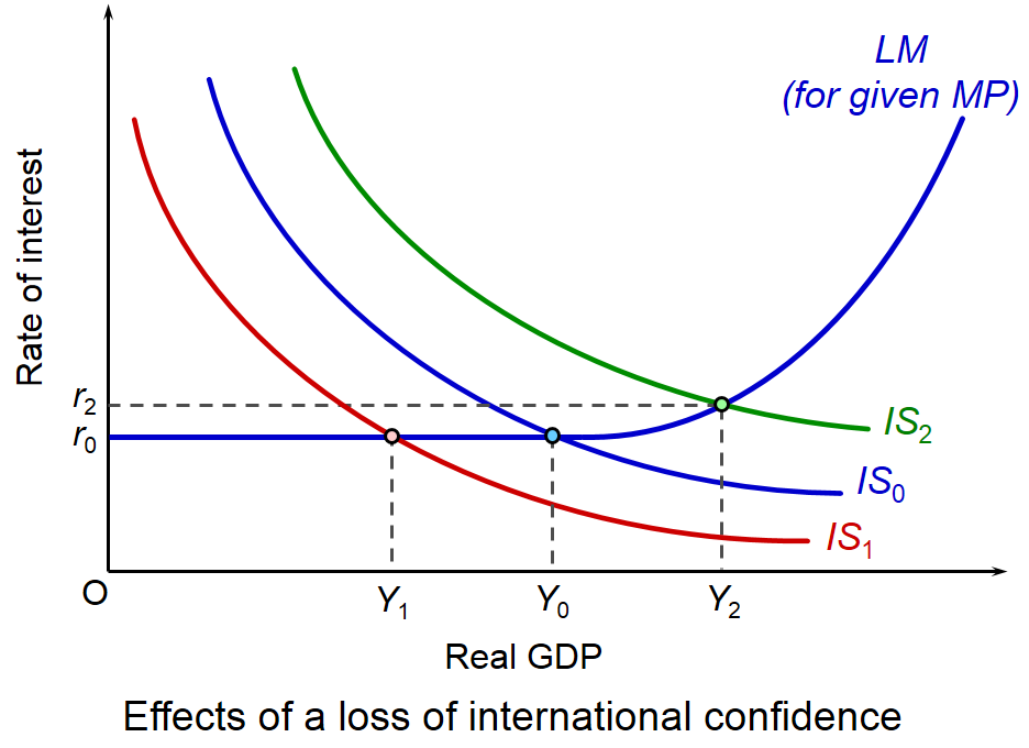
Paul Krugman and Simon Wren-Lewis challenge Rogoff’s arguments. Paul Krugman uses a version of the IS-LM model to analyse the effect of a loss of international confidence in the UK following problems in the eurozone and worries about excessive UK borrowing.
In the model, the LM curve (labelled MP in Krugman’s diagrams) illustrates the effect of an increase in real GDP on interest rates with a particular monetary policy (e.g. an inflation target or a Taylor rule, which involves a mix of two policy objectives: an inflation target and real GDP). As GDP rises, putting upward pressure on inflation, so the central bank will raise interest rates. Hence, like the traditional LM curve, the monetary-policy related LM curve will slope upwards, as shown in the diagram.
Initial equilibrium GDP is Y0. The rate of interest is at the minimum level, r0 (i.e. the rate of 0.5% that the Monetary Policy Committee has set since January 2009). This, in the model, is the liquidity trap, where any increase in money supply (a rightward shift in the LM curve) will have no effect on interest rates or GDP.
In Rogoff’s analysis of a crisis triggered by excessive borrowing and problems in the eurozone, the IS curve will shift to the left (as illustrated by curve IS1) as capital flows from the UK and confidence collapses. Real GDP will fall to Y1. This will be the outcome of fiscal expansion in the world of the early 2010s.
Krugman argues that the opposite will occur. The outflow of capital will drive down the exchange rate. This will lead to an increase in exports and a decrease in imports. Aggregate demand thus rises and the IS curve will shift to the right (e.g. to IS2 in the diagram. Real GDP will rise (e.g. to Y2 in the diagram). If the rise in aggregate demand is sufficient, the economy will rise out of the liquidity trap and interest rates will rise (e.g. to r2 in the diagram).
Not surprisingly, Rogoff challenges this analysis, as you will see if you read his second paper below. He doesn’t criticise the model per se, but challenges Krugman’s assumptions. For example, a depreciation of sterling by some 20% since 2008 doesn’t seem to have had a major effect in stimulating exports (see the chart in the news item, A balancing act). And exports could well have declined if the eurozone economy had collapsed, given that exports to the eurozone account for around 44% of total UK exports.
Rogoff’s assumptions in turn can be challenged. Simon Wren-Lewis argues that, provided a credible long-term plan for deficit reduction is in place, maintaining a fiscal stimulus in the short run, to keep the recovery going that was beginning to emerge in 2010, would help to increase investor confidence, not undermine it. And, with a policy of quantitative easing, which involves the Bank of England buying central government debt, there is no problem of a lack of demand for UK gilts by the private sector.
What is clear from this debate is the willingness of both sides to accept points made by the other. It is an extremely civilised debate. In fact, it could be seen as a model of how academic debate should be conducted. There is none of the ‘shouting’ that has charaterised much of the pro- and anti-austerity lobbying since the financial crisis burst onto the world stage.
Explain how the policy-dependent LM curve illustrated in the diagram is derived.
What would cause the policy-dependent LM curve to shift?
Explain what is meant by the ‘liquidity trap’. Why does being in a liquidity trap make monetary policy ineffective?
How would you determine whether or not the UK is currently in a liquidity trap?
How is the level of (a) public-sector debt and (b) private sector debt owed overseas likely to affect the confidence of investors concerning the effects of an expansionary fiscal policy?
In an interview with the Yorkshire Post, Mark Carney, Governor of the Bank of England, said that under current circumstances he did not feel that further quantitative easing was justified. He said:
My personal view is, given the recovery has strengthened and broadened, I don’t see a case for quantitative easing and I have not supported it.
In response to his speech, the pound strengthened against the dollar. It appreciated by just over 1 cent, or 0.7%. But why should the likelihood of no further quantitative easing lead to a strengthening of the pound?
The answer lies with people’s anticipation of future interest rates. If there is no further increase in money supply through QE, interest rates are likely to rise as the economy recovers and thus the demand for money rises. A rise in interest rates, in turn, is likely to lead to an inflow of finance into the country, thereby boosting the financial account of the balance of payments. The increased demand for sterling will tend to drive up the exchange rate.
However, an increase in aggregate demand will result in an increase in imports and a likely increase in the balance of trade deficit. Indeed, in July (the latest figures available) the balance of trade deficit rose to £3.085bn from £1.256bn in June. As recovery continues, the balance of trade deficit is likely to deteriorate further. Other things being equal, this would lead to a depreciation of the pound.
So if the pound appreciates, this suggests that the effect on the financial account is bigger than the effect on the current account – or is anticipated to be so. In fact, given the huge volumes of short-term capital that move across the foreign exchanges each day, financial account effects of interest rate changes – actual or anticipated – generally outweigh current account effects.
Explain how quantitative easing affects exchange rates.
What is happening concerning quantitative easing in the USA? How is this likely to affect the exchange rate of the US dollar to sterling; other currencies to sterling?
Why may an increase in the balance of trade deficit lead directly to an appreciation of the exchange rate?
Why is an anticipation of a policy change likely to have more of an effect on exchange rates than the actual policy change itself? Why, indeed, may a policy change have the reverse effect once it is implemented?
Under what circumstances may speculation against exchange rate changes be (a) stabilising; (b) destabilising?
How is quantitative easing (or an anticipation of it) likely to affect each of the main components of the current and financial accounts of the balance of payments?
For what reasons might sterling have been ‘overbought’ and hence be overvalued?
What is meant by the real exchange rate (REER)? Why may reference to the REER suggest that sterling is not currently overvalued?
 When the rest of the developed world went into recession after the financial crisis of 2007/8, the Australian economy kept growing, albeit at a slightly lower rate (see chart 1: click here for a PowerPoint). Then as the world economy began to grow again after 2009, Australian grow accelerated. Partly this was the result of a strong growth in demand for Australian mineral exports, such as coal, iron ore and bauxite, especially from China and other east Asian countries.